
jol /

experimental research / optical measurements

jonathan oliveira luiz

experimental mechanics
optical metrology
biomechanics & acoustics
vibrations

01 / research & engineering

projects

fieldsexperimental mechanics
optical metrology
biomechanics
acoustics
vibrations
laser processing
instrumentation & softwareoptomechanical design · synchronized acquisition · external triggering · phase reconstruction · full-field mapping · time- and frequency-domain analysis
01cochlear micromechanics

Depth-resolved measurements of nanometer-scale responses, traveling waves and localized mechanical properties using acoustic and pulsed-laser excitation.

methods / spectral-domain OCT · phase-sensitive vibrometry · OCE · thermoelastic excitation · laser-induced air sparks

02middle-ear dynamics

Full-field characterization of nonlinear middle-ear transfer functions and impulse responses across sound pressure levels.

methods / high-speed stereo 3D-DIC · LDV · acoustic excitation · signal processing · 3D-printed models

03blast loading & damage mechanics

Dynamic response, fracture and fluid–structure interactions of human tympanic membranes under blast exposure.

methods / shock tube · high-speed imaging · Schlieren · 3D-DIC · pressure measurements

04residual stress metrology

Residual stress characterization in cross-sections of small parts by combining the contour method and scanning white-light interferometry.

methods / contour method · scanning white-light interferometry

Experimental Mechanics / 2022

05laser processing & nondestructive testing

Picosecond laser microstructuring of filters for oil/water separation and surface characterization.

methods / picosecond laser ablation · microscopy · wettability characterization

06shearography / SHIC

Shearography for nondestructive inspection of composite materials. My work included optomechanical design and assembly, interferometer testing, vibration sensitivity studies, and software for control and optical data analysis.

methods / shearography · interferometry · optomechanical design · vibration testing

07annelida / mechanical design

Mechanical design and prototype evaluation for a robot developed to unclog pipelines in the oil industry at SENAI.

methods / component design · numerical structural analysis · optimization · prototype validation

me / researcher & engineer

jonathan oliveira luiz

I am a mechanical engineer and Ph.D. candidate at Worcester Polytechnic Institute, working at the intersection of experimental mechanics, optical metrology and biomechanics.

My work combines optical instrumentation, custom acquisition and analysis software, and experiments on middle- and inner-ear mechanics, in collaboration with Massachusetts Eye and Ear and Harvard Medical School.

My work also includes acoustics and vibrations, from middle-ear impulse responses to optical measurements of motion.

Previously, I worked on residual stress measurement, laser processing, nondestructive testing and mechanical design. I also teach engineering and experimental measurement methods.

Jonathan Oliveira Luiz

contact & links

02 / curriculum vitae

Research assistant and Ph.D. candidate in Mechanical Engineering at WPI. Optical metrology and biomechanics research in collaboration with Massachusetts Eye and Ear and Harvard Medical School.

education

2023–present

Ph.D. / Mechanical Engineering

Worcester Polytechnic Institute · optics and acoustics
Advisor: Cosme Furlong

2019–2021

M.Sc. / Mechanical Engineering

Federal University of Santa Catarina · optical metrology
Advisor: Armando Albertazzi

2018

study abroad / laser processing

University of Bremen

2013–2019

B.S. / Mechanical Engineering

Federal University of Santa Catarina

research & engineering

2023–present

CHSLT / WPI

Graduate research assistant · optical metrology and biomechanics

2021–2022

SENAI / Annelida

Mechanical design, structural analysis and prototype evaluation

2019–2021

LABMETRO / UFSC

Graduate research assistant · residual stress measurement and optical metrology

2018

BIAS / Bremen

Research intern · picosecond laser ablation for oil/water separation

2015–2017

LABMETRO / UFSC

Undergraduate research assistant · shearography for nondestructive inspection of composites

journal articles

Active Anti-Fogging in Transparent Media by Ultrasonic ExcitationD. Ruiz-Cadalso, A. Salerni, H. Zheng, J. O. Luiz, D. Ziegler, C. Furlong · Experimental Mechanics · 66, 175–192 · 2026
Quantifying Real-Time Dynamic Responses and Damage Mechanics of Human Tympanic Membranes Exposed to Blast WavesJ. Oliveira Luiz, A. Alipanahi, J. J. Rosowski, C. Furlong, J. T. Cheng · ASME JESMDT · 8(4), 041106 · 2025
Residual Stress Characterization in Cross-Sections of Small Parts by Combining the Contour Method and Scanning White-Light InterferometryJ. Oliveira Luiz, M. R. Viotti, A. Albertazzi Jr. · Experimental Mechanics · 62, 1333–1348 · 2022

manuscripts in preparation

Time-Domain Responses of the Human Middle Ear to Clicks and Blasts Using Full-Field High-Speed 3D-DIC and 1D Laser-Doppler Vibrometrymanuscript in preparation

conference proceedings & presentations

teaching

2026

Stress Analysis

Instructor · first five lectures · WPI

Laser Metrology and Nondestructive Testing

Guest lecturer and laboratory instruction support · WPI

2023

Integrated Thermomechanical Design and Analysis

Guest lecturer · WPI

2014

mathematics for engineering

Undergraduate teaching assistant · UFSC

selected awards & outreach

G. L. Cloud Scholarship Award / SEM / 3rd place / 2025
MidWinter Meeting Travel Award / ARO / 2025
SPIE UFSC Student Chapter / president / 2017
Einstein Floripa / volunteer mathematics teacher / 2020

blog /

01 / interference · draft

why does a soap bubble show colors?

As a child, I used to wonder about the colorful oil stains on asphalt after the rain. Where did those colors come from?
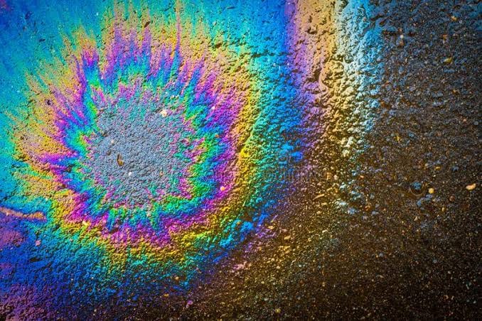
Rainbow-colored oil film on asphalt
oil on asphalt / a question about light

Years later, I explored the same question with a soap film. What was light doing inside such a thin layer?

01 / light, waves & interference

Light is an electromagnetic wave: electric and magnetic fields oscillate as it travels. Wavelength is the distance between repeating peaks. Different visible wavelengths correspond to different spectral colors; white light contains many wavelengths. The drawings below follow the electric field.

Phase tells us where a wave is within its cycle. Waves can have the same wavelength and amplitude while their peaks arrive at different times. One full cycle is 360° or 2π radians.

When two light waves overlap, their electric fields add. Waves in phase reinforce each other: constructive interference. Waves half a cycle apart cancel when their amplitudes are equal: destructive interference.

Equal-amplitude monochromatic waves with the same polarization. The curves show electric field, not intensity; the intensity readout is time-averaged and normalized.

02 / two reflections, one film

Light reflects at both surfaces of the film. The reflected waves travel different optical paths before they meet. Their relative phase determines whether they reinforce or cancel each other.

The response depends on wavelength. A thickness that suppresses one wavelength may reflect another more strongly. Under broad-spectrum illumination, that changes the balance of reflected colors.
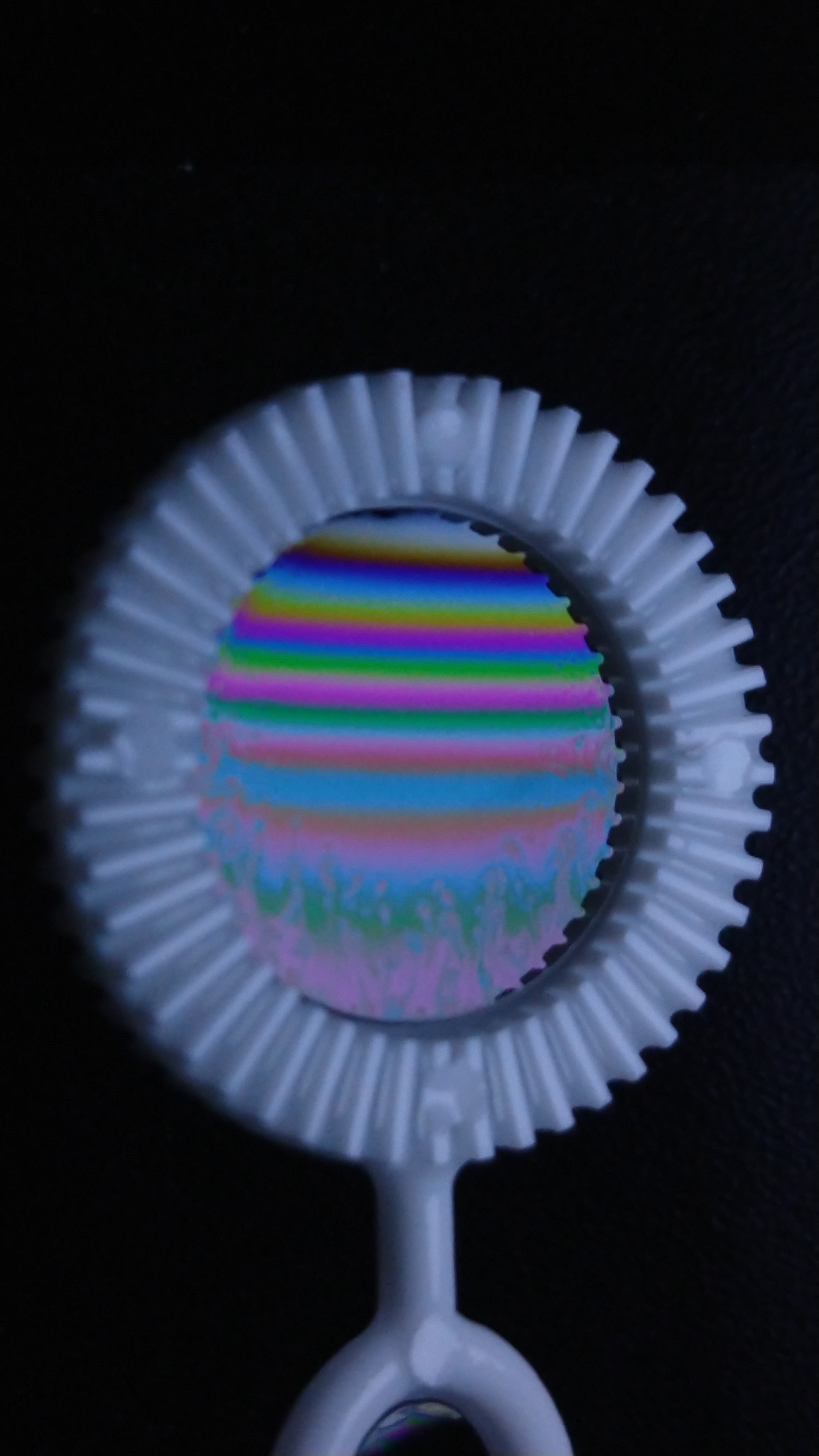
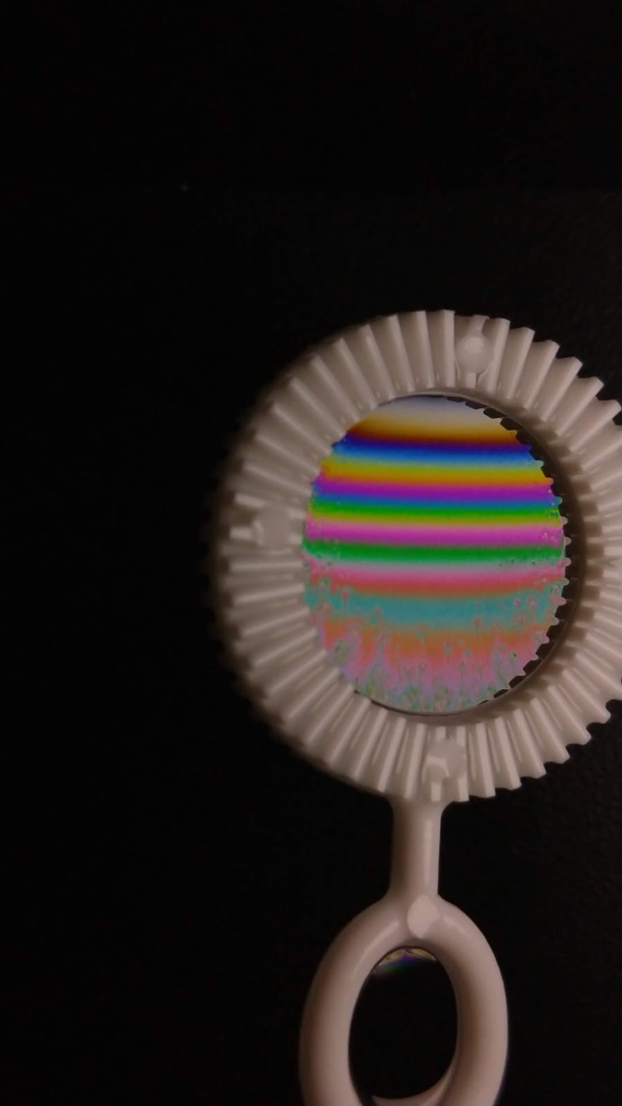
Soap film in a circular holder, showing horizontal colored interference bands
soap film experiment / 2019

03 / what changes when the film gets thinner?

Same film, different wavelengths. The extra optical path and the phase reversal at the first reflection determine how the reflected waves combine. Geometry is exaggerated.

Move the thickness control. Follow the three curves and watch how their balance changes.

350 nm
three-channel preview

Illustrative air–film–air model: n = 1.33, normal incidence, wavelengths 648 / 552 / 453 nm. The color preview uses normalized channels to make the changes visible. It is not a calibrated white-light color prediction.

04 / why do the colors repeat?

Changing the thickness changes the relative phase of the reflected waves. Reinforcement and cancellation repeat, but at different thicknesses for each wavelength. The mixture of reflected wavelengths creates the colored bands.

In a 2019 interferometry course project, Claudio Ramos Schmitz and I photographed a soap film with a smartphone to study this response. The colors became a visible trace of the interference between its two reflections.

05 / can interference become a measuring tool?

In the soap film, a change in optical path changes the phase and the reflected colors. Could we arrange those paths deliberately, compare an object with a reference and turn interference into a measurement?

references

Afanasyev, Andrews & Deacon / Measuring soap bubble thickness with color matching / 2011

Atkins & Elliott / Investigating thin film interference with a digital camera / 2010

Kitagawa / Thin-film thickness profile measurement by three-wavelength interference color analysis / 2013

blog /

02 / interferometry · draft

can a photograph measure depth?

A picture tells us how bright each pixel is. A depth map tells us where the surface is. How can a camera measure the second quantity when it only records the first?

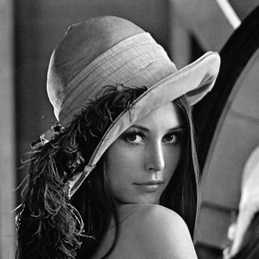
Lenna photograph supplied as an intensity-image example
A photograph records the light reaching each pixel: brightness and color. It does not directly attach a measured distance to that pixel.

Photography has long let us record how a scene looks. Perspective, focus and shading can suggest depth, but a conventional photograph records intensity. Could we also record the information carried by the phase of light?

2D image / one fixed view

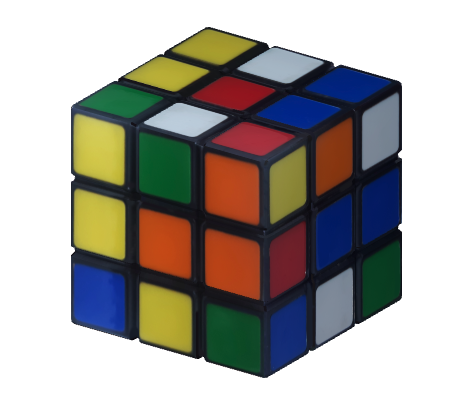
Fixed two-dimensional render of the same Rubik’s cube model
At P, the image records color and brightness, not a depth value.

3D model / explore the geometry

near / 0relative depthfar / 1
Same object and initial viewpoint. Rotate to reveal other faces.

Look at point P. The left image tells us its color and brightness. The right model also tells us where it is in space: the same point has a depth value. The color scale makes that extra information visible. How could we measure it using light?

Shape and shading in a picture can suggest depth, but do not directly record a distance for each point. Both views here use a supplied model; the left is a render, and the right is not reconstructed from it. Depth is normalized to 0–1 in a fixed reference range, not a physical measurement. A hologram encodes wavefront information through interference with a reference.

01 / using light to measure depth

revisit / light, phase & interference in a soap film

In the soap film, light reflected along two paths and the waves added. Here we arrange those paths deliberately: one visits the object, the other a known reference. Their phase difference becomes an intensity pattern. If we can recover that phase, we can measure how far light traveled.

For a narrow-spectrum source, a stable relative phase produces persistent bright and dark fringes. This stability is coherence. Move the relative phase below, then compare it with a phase that fluctuates during the camera exposure.

Equal beams with matched polarization. The fluctuating case averages uniformly over a full phase cycle during one exposure. It illustrates lost mutual coherence, not a literal animation of broadband light.

02 / how do optical paths become a height measurement?

A beam splitter sends light to the object and a reference mirror. Their returning waves meet at the camera. A difference in path changes their phase; interference makes that difference visible as bright and dark fringes.

Δφ = 2π ΔOPD / λ

In reflection in air, the light travels to the surface and back: a height change Δh changes the path by 2Δh.

compare four known phase offsets

camera frames → recovered phase → height

Move the reference mirror: the fringes shift, while the object stays in place. Comparing four frames with known phase shifts separates the object phase from the brightness. The recovered height should stay the same.

Ideal simulation at 632.8 nm. The small camera frame repeats the middle panel. Four frames with 0°, 90°, 180° and 270° additional shifts are synthesized at each reference position; the known reference tilt and offset are removed. Height stays within one reflection phase cycle. Object shape and mirror motion are exaggerated in the diagram.

03 / why does phase wrap?

Phase repeats every 2π. As the surface rises, the true phase keeps increasing, but the recovered angle returns to the interval −π to +π. The jump belongs to the representation, not necessarily to the surface.

Unwrapping counts the missing cycles by following a continuous phase field. Real steps, noise and undersampled fringes can make that count ambiguous. In reflection in air, an extra λ/2 of height adds a full phase cycle.

A camera can reveal hidden information when we change how light reaches it. Before returning to surface measurements, can we use light to see the air itself?

previous / the soap film experiment
blog /

03 / flow visualization · draft

can we see air?

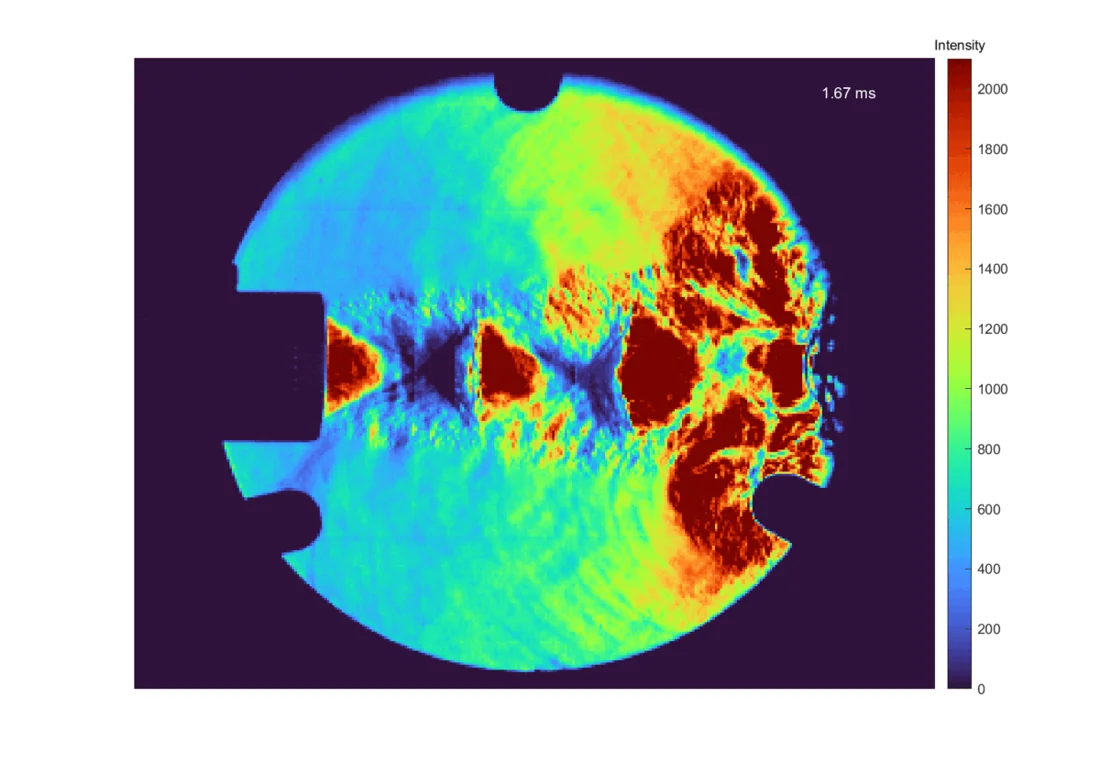
We feel a breeze, but the air itself is usually invisible. What changes when a shock wave passes through it? These shock-tube recordings show how an optical arrangement can turn changes in the air into an image.

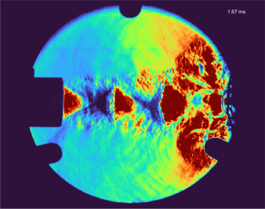
High-speed shock-tube recording
Shock-tube experiment / schlieren intensity rendered in color. The original intensity scale and time labels are retained.
Web preview sampled from the original GIF. Playback speed is a viewing control; the time labels inside the recording describe the experiment.

01 / how does schlieren reveal air?

When air density changes, its refractive index changes too. A density gradient bends light slightly. Collecting optics focus the light at a knife edge. Deflected rays shift the source image relative to the edge, changing how much light reaches the camera. Color schlieren uses a color-selective cutoff instead. We see optical evidence of the density variations, not the air molecules themselves.

Simplified lens-based schlieren arrangement. The knife edge lies in the focal plane of the collecting lens. Camera imaging optics are omitted. Ray angles and brightness are illustrative; this is not a calibration of the recordings.

A shock front produces a sharp change in the flow. Watch for a moving boundary in the optical view, then follow how the pattern evolves. Brightness and color are not a calibrated pressure map here.

02 / what does a picture leave out?

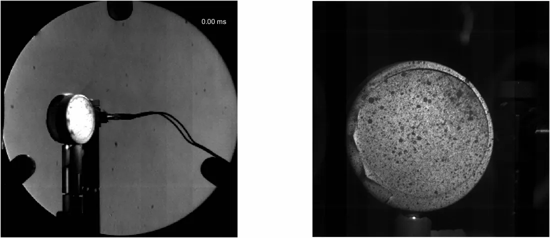
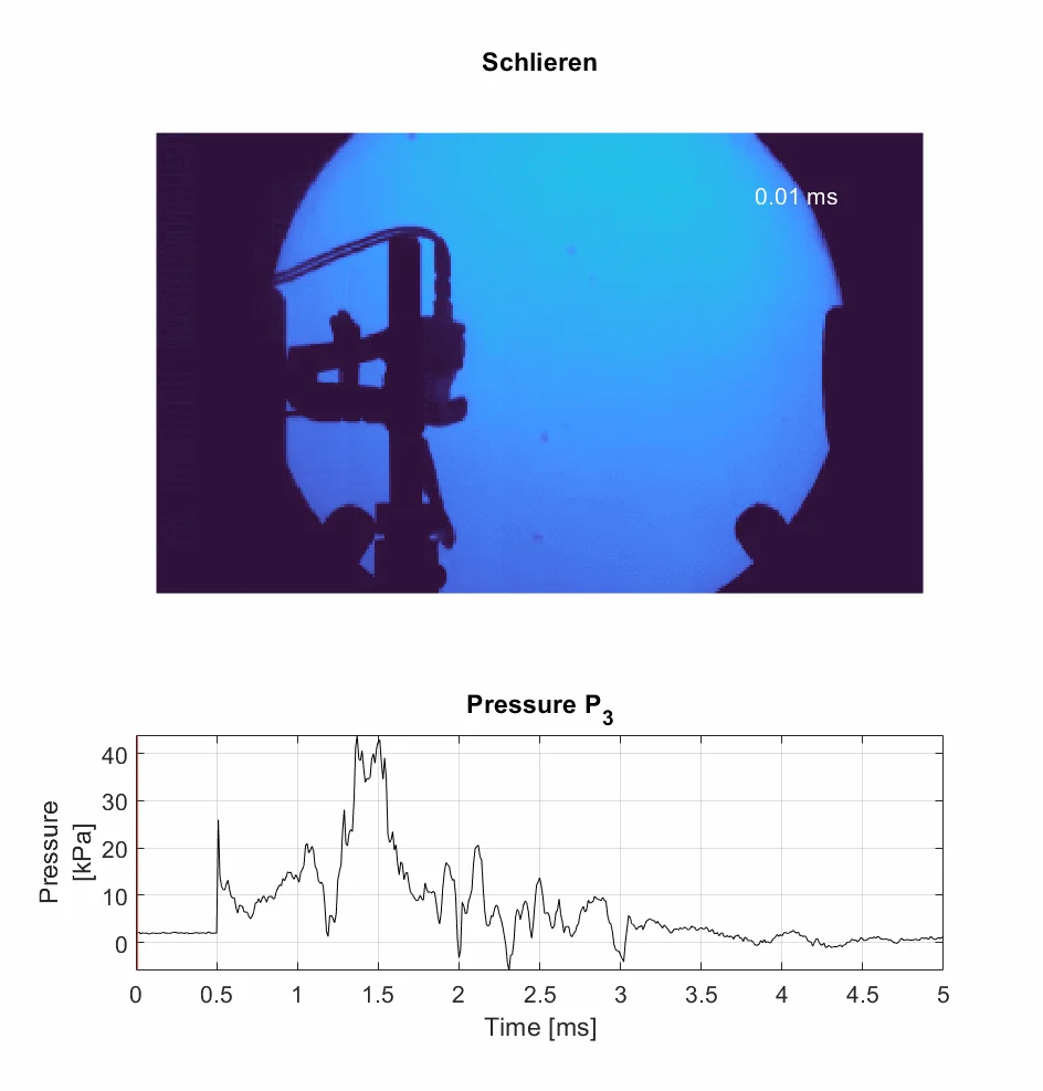
The optical sequence tells us where structures appear and how they move. Pressure sensors add a different measurement: pressure over time at their locations. Their combination is more informative than either alone, but we still need the setup, calibration and sensor positions before making quantitative claims.

High-speed shock-tube recording
Schlieren and membrane rupture / two recorded views of the same experiment. Preview limited to the first 450 source frames.
Web preview sampled from the original GIF. Playback speed is a viewing control; the time labels inside the recording describe the experiment.
High-speed shock-tube recording
Schlieren and measured pressure / the ARO recording preserves the P₃ pressure trace and its moving time cursor. This is a separate experiment from the rupture sequence above.
Web preview sampled from the original GIF. Playback speed is a viewing control; the time labels inside the recording describe the experiment.

03 / what keeps a wing up?

Around a lifting wing, the pressure distribution produces a net upward force and the airflow is deflected downward. Bernoulli relates speed and pressure in a simplified steady, low-speed flow. It helps interpret a known flow field; it does not determine that field by itself.

p + ½ρv² = constant

Qualitative wing sketch, not a CFD solution. The pressure readout uses a chosen local speed, air density 1.225 kg/m³ and a reference speed of 40 m/s. It is not a lift prediction or a measurement from the GIFs.

Use this form along a streamline with constant density, negligible viscous losses and height changes. It is not the equation for the shock front in the recordings above. Air parcels above and below a wing do not have to meet at the trailing edge at the same time.

04 / seeing is the start of measuring

Flow visualization turns an invisible event into something we can inspect. Schlieren, particle-based methods and interferometry reveal different quantities. The next post returns to surface shape: how can white light locate a surface rather than just show a pattern?

references

Experimental material from my shock-tube work, including the schlieren sequence in my ARO presentation. Web previews preserve the source labels; setup details, sensor locations and a fuller interpretation will follow.

NASA Glenn / Schlieren flow visualization

NASA Glenn / Bernoulli’s equation · Bernoulli & Newton


previous / photography & phase
blog /

04 / white-light interferometry · draft

how can white light measure shape?

A single wavelength let us recover phase, but its cycles repeat: different heights can give the same phase. Can a broad spectrum tell us which height we are looking at? By scanning a known reference position, we will recover a depth at each pixel and assemble the shape of a surface.

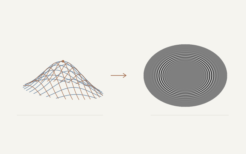
Simulation / the curved profile and fringes come from the same surface. P marks its center in both views.
This is a teaching simulation, not experimental footage. The surface and optical model are known; the experiment below explains how envelope maxima recover the shape.

01 / what does coherence mean?

Temporal coherence describes how well a light field remains correlated with a delayed copy of itself. A narrow spectrum maintains that correlation over a longer optical-path difference. A broad spectrum loses it sooner.

Temporal coherence only. Gaussian spectrum in wavenumber, centered at 840 nm. Colored curves illustrate three spectral components; the envelope includes the continuous spectrum. Colors identify curves, not visible light.

Light often called “incoherent” can still interfere with a copy of itself when the delay is short enough. White-light interferometry uses this limited coherence. Spatial coherence is a separate requirement of the optical arrangement.

02 / how can an envelope maximum reveal depth?

A motorized stage moves the reference mirror to known positions. At every position, the camera records the intensity at every pixel. Move the stage manually or run a scan; each pixel stores the position where its envelope is strongest.

light sourcebeam splittersurfacecamera / one pixelreference mirrorcontrolled stage

Same object, same points. The surface model is shown in perspective; the measured map is viewed from above.

Automatic scan: 0.10 µm stage steps. The reconstructed values are sampled peak positions, relative to the calibrated reference plane.
choose a surface point

The vertical cursor is the current stage position. A, B and C have different peak positions. Their depth comes from the calibrated stage coordinate at each peak, not from the pixel brightness alone.

one maximum per pixel → a surface map

The map updates as the scan collects positions. Unconfirmed pixels stay gray; confirmed depths are colored. One scan samples the whole camera field, rather than measuring A, B and C one at a time.

Simulated surface, 64 × 32 pixels. Depth is relative to a reference plane; this illustrates the reconstruction, not an experimental result.Ideal equal-intensity beams, one surface, no noise. Broadband model: Gaussian spectrum in wavenumber, centered at 840 nm, approximately 50 nm FWHM. This is infrared light; curve colors identify wavelengths only.

The mirror moves by Δz, but light travels that distance twice: the optical path difference changes by 2Δz. With broadband light, interference contrast is concentrated near equal optical paths. The maximum of the envelope identifies the depth of the selected point. Repeating this for every pixel maps the surface; a single fringe does not identify a unique position.

03 / what can we do with the measured surface?

A depth at every measured pixel gives a surface topography: steps, curvature and tiny changes in shape. What if those changes appeared after cutting a metal part?

previous / seeing air
blog /

05 / the contour method · draft

how can a measured surface reveal stress?

The previous post turned interference into a surface map. What if that surface changed because we cut a stressed metal part? The contour method uses the released deformation to reconstruct the stress component normal to the cut. Here we follow the method; the next post tests it and applies it to offshore riser wires.

Finite-element wire model with a prescribed surface displacement field
The measured surface becomes a displacement boundary condition on a finite-element model. The elastic calculation recovers stress.

01 / what changes when we cut a stressed part?

Cutting releases traction on the new surfaces. Under elastic relaxation, their tiny changes in shape contain information about the stress component normal to the cut.

Conceptual sequence. Deformations are exaggerated; colors are illustrative, not experimental stress values.

02 / how does a surface become a stress map?

Align, mirror and average the two cut faces. Carefully smooth the contour, then use it to reconstruct the stress component normal to the cut.

two cut facesalign & averagesmoothelastic modelnormal stress

why measure both cut faces?

Conceptual profiles with exaggerated displacements. Averaging cancels opposite artifacts; common artifacts can remain.

The interferometer measures surface geometry. The contour method provides the mechanical reconstruction. Cutting quality, roughness and smoothing affect the result.

03 / why are small parts difficult to measure?

Roughness and measurement noise can obscure the small elastic relaxation. Their rapid spatial variations can also be amplified in the stress calculation.

how much smoothing is enough?

Try smoothing this synthetic profile. Too little leaves rapid fluctuations; too much removes a real, localized feature along with the noise.

gray / measured · blue dashed / true shape · black / smoothed

Synthetic example: the true shape is known. For real measurements, choose smoothing through stability, uncertainty and validation.

04 / how do displacements become stresses?

In a linear elastic finite element model, we reverse the measured relaxation to restore the cut face to a plane. The stresses needed to do this reconstruct the original normal residual stress.

Illustrative profile and mesh. Arrows show prescribed displacements, not applied forces. The interior response and stresses require an elastic finite element solve; this diagram does not run that solver.
see the specimen mesh

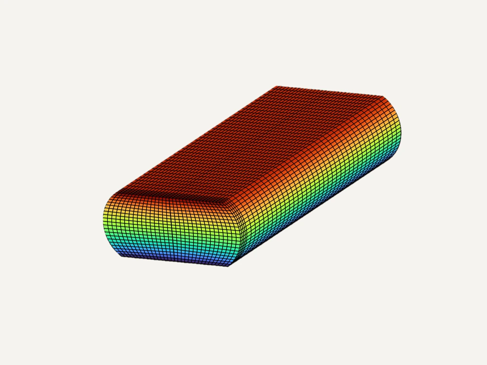
finite element mesh / wire specimen

Wire specimen mesh. Select to enlarge.
un|cut = −ūs

uₙ is displacement normal to the cut; ūₛ is the averaged, smoothed relaxation. The minus sign reverses that relaxation.

The model uses the specimen geometry, Young’s modulus and Poisson’s ratio, with constraints to prevent rigid-body motion. It assumes elastic relaxation during cutting.

05 / where does this become useful?

We now have the chain: measured surface → processed displacement → elastic model → normal stress. Next, we look more closely at the data-conditioning choices in that chain. Then we validate the method against a known stress field and investigate riser wires.

references

Luiz, J. O. / Medição de tensões residuais em arames de risers flexíveis associando o método do contorno à interferometria de luz incoerente / UFSC, 2021.

Oliveira Luiz, Viotti & Albertazzi Jr. / Residual Stress Characterization in Cross-Sections of Small Parts By Combining the Contour Method and Scanning White-Light Interferometry / 2022

previous / white-light interferometry
blog /

06 / noise · draft

what is noise?

A camera records light. A microphone records pressure. Both can capture the response we want and fluctuations we did not ask for. How do we tell them apart?

01 / noise depends on the question

In a measurement, noise is unwanted variability that obscures the quantity of interest. A vibration can be the signal when we study a structure, or a disturbance when it moves an optical setup. Noise need not be fast, random or acoustic; high frequency alone does not make something noise.

02 / optics & acoustics

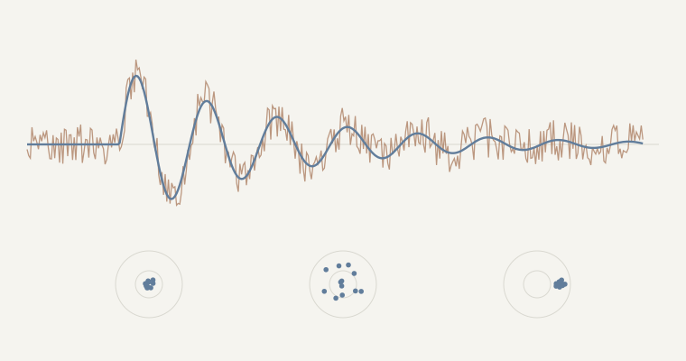
In optical measurements, fluctuations in detected light and camera electronics can affect intensity and the phase we recover. In acoustic measurements, background sound and sensor electronics can obscure pressure or vibration. The mechanisms differ; the practical question is the same: how much of this record belongs to the response?

Illustration with a repeatable signal and independent, zero-mean additive noise. Units and amplitudes are normalized. Averaging assumes the response is aligned and unchanged between records; it does not remove systematic offsets or correlated disturbances.

03 / precise, but accurate?

Each point is a repeated measurement; the center is the known reference. Precision describes how closely the measurements agree with one another. Accuracy describes closeness to the true value. A tight cluster away from the center is precise, but its measurements are systematically wrong.

Synthetic measurements in arbitrary units. Random errors vary between observations; a systematic component stays fixed here. A centered mean alone does not make scattered individual measurements accurate. Closeness of the mean to the reference is called trueness; precision concerns dispersion. In real experiments, the true value is generally unknown and we use a reference with its own uncertainty.

Repeating and averaging can reduce independent random fluctuations. They do not correct a fixed systematic error. That requires investigating the instrument, method or calibration—the same distinction behind the fixed-offset control above.

04 / noise in human judgment

In Noise: A Flaw in Human Judgment, Daniel Kahneman, Olivier Sibony and Cass R. Sunstein examine unwanted variability in judgments that should agree. Bias shifts judgments systematically; noise makes them inconsistent. This is an analogy to measurement, not the same physical mechanism. A stable result can still be wrong, and a variable result needs more than a prettier curve.

05 / before reaching for a filter

First define the signal, inspect repeated records and check the instrument and environment. Reduce disturbances at the source when possible. Averaging and filtering answer different questions: one combines repeated observations; the other changes which variations remain in a record. The next draft explores when smoothing removes noise and when it removes useful shape.

references

BIPM / accuracy, trueness & precision (VIM)

Kahneman, Sibony & Sunstein / Noise: A Flaw in Human Judgment / 2021

Hamamatsu / camera signal-to-noise ratio

NIST / measurement uncertainty


previous / the contour method
blog /

07 / data conditioning · draft

how much smoothing is too much?

A measured surface contains more than the deformation we want. How do we reduce noise without erasing the shape that carries the stress information?

01 / shape, texture or noise?

The recorded profile combines overall form, waviness, roughness and measurement errors. Cutting can add artifacts too. A rapid variation is not automatically noise: its meaning depends on the measurement and the engineering question.

02 / the same signal, two views

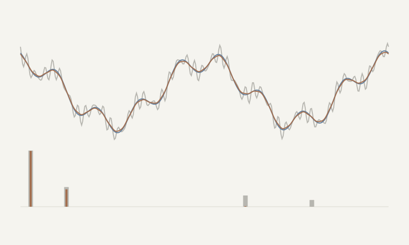
A profile shows where a variation occurs. Its frequency spectrum shows the scales of those variations. For a surface, we use position and spatial frequency (cycles/mm). For a time record, the equivalent axes are time and frequency (Hz). These are two views of the same data, not two different measurements.

Synthetic periodic profile with two shape components and two added disturbances. Gaussian low-pass illustration; the reference shape is known here, unlike a real measurement. High spatial frequency alone does not identify noise.

03 / less noise, or less information?

Move the filter scale. A weak filter leaves fast oscillations. A strong filter also suppresses the smaller real feature. The useful setting preserves the relevant shape while reducing disturbances; it is not simply the smoothest curve.

04 / what did we do in the wire measurements?

Before smoothing, the two cut faces must be aligned, mirrored and averaged. Averaging cancels antisymmetric cutting effects, but symmetric artifacts can remain. Outliers and local cutting defects require separate inspection; smoothing is not a universal repair.

splines

Fit a smooth surface. Knot spacing controls the detail retained; too much spacing can erase form.

patch fitting

The dissertation adapts smooth fitting to irregular meshes using overlapping polynomial patches.

Gaussian filtering + interpolation

Filter the displacement field, then interpolate it onto the FEM mesh. Pay attention to edges, steps and outliers.

The smoothing choice propagates into the calculated stress. Compare stable features, edge behavior and uncertainty as the smoothing changes. The dissertation discusses selecting smoothing from the reconstructed stress response; no single setting works for every surface.

references

Luiz, J. O. / Medição de tensões residuais em arames de risers flexíveis associando o método do contorno à interferometria de luz incoerente / UFSC, 2021.

Residual Stress Characterization in Cross-Sections of Small Parts By Combining the Contour Method and Scanning White-Light Interferometry / 2022


previous / understanding noise
blog /

08 / offshore risers · draft

what is hiding inside a wire?

A flexible riser connects subsea equipment to a floating production platform. Its failure can interrupt production, require replacement and release fluids. Reliability depends on small metallic wires hidden inside the pipe. What can optical measurements reveal about their internal stress?

01 / from the whole riser to one wire

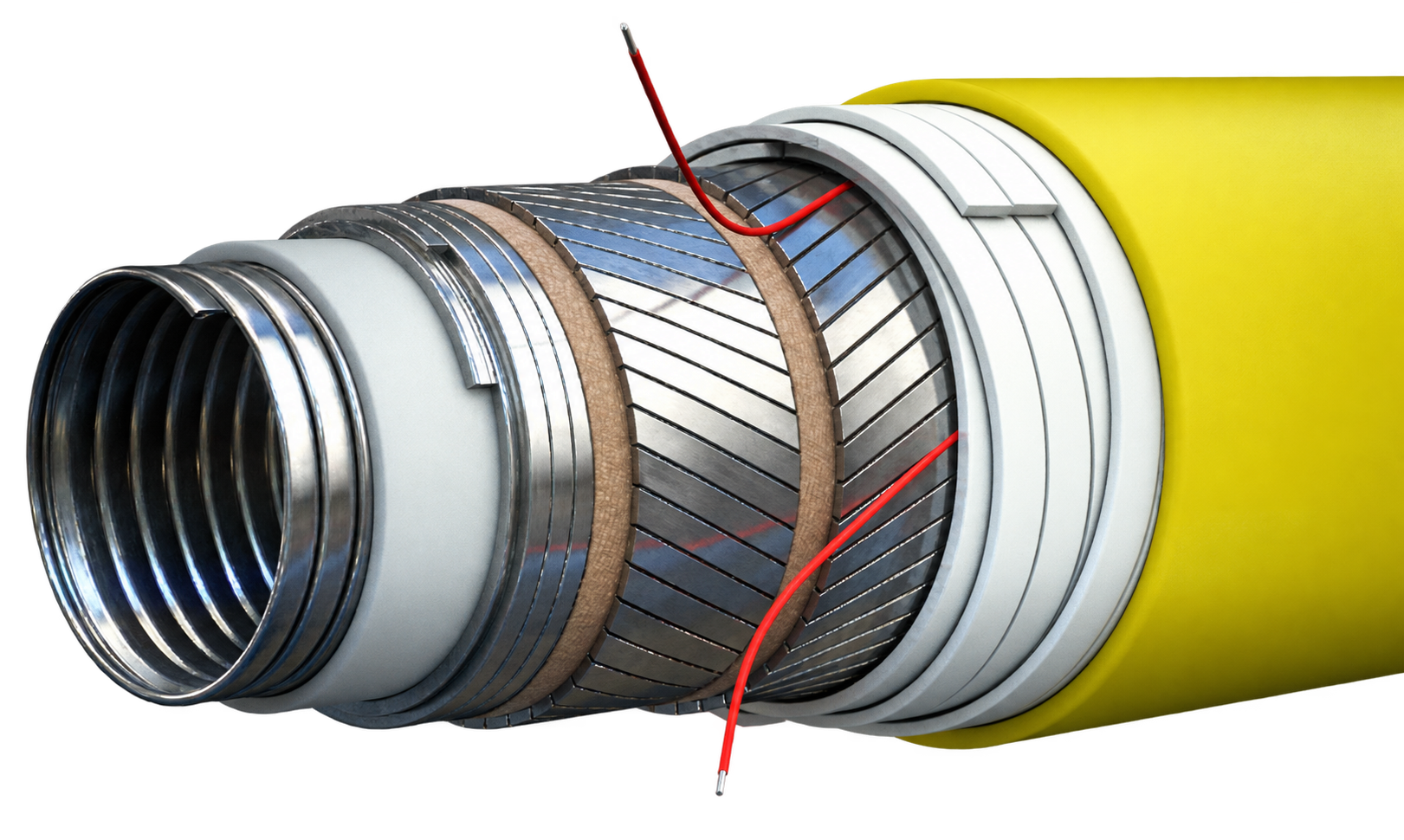
The pipe contains polymer and metal layers with different jobs. Tensile-armour wires wind around it in opposing helices, carrying axial loads. Manufacturing and forming can leave residual stresses before the riser ever enters service. Those stresses combine with the stresses produced by operational loads.

Cutaway of a flexible pipe with opposite helical tensile-armour layers
A flexible pipe is a layered structure. The helical armour wires carry loads as the floating unit and the sea move.
Flexible-pipe illustration reproduced from the supplied dissertation presentation; original credit: Journal of Petroleum Technology.

Simplified schematic inspired by my dissertation and defense presentation. Layers, wire size and deformation are not to scale; colors in the section are conceptual. Experimental stress maps follow below.

In my master's research, I combined scanning white-light interferometry with the contour method to measure this normal stress component in small wire cross-sections. The optical measurement supplies the relaxed surface shape; the elastic model supplies the stress. First, we check the method against a controlled bending test.

revisit / the contour method

02 / can the method recover a known bending profile?

revisit / conditioning measured data

A normalized steel bar (6 × 19 mm) was bent beyond yield and unloaded. We compare the measured residual stresses with the analytical bending profile.

how was a residual stress field created?

Qualitative sequence with exaggerated curvature. The maps below are experimental results.

After unloading, the remaining stress is the loading profile minus the elastic stress released. This subtraction produces the alternating tensile and compressive bands.

σres(y) = σload(y) − My/I

M is the applied bending moment, I the section’s second moment of area, and y the distance from the neutral axis. The loading profile includes yielding; My/I alone describes elastic bending, not the residual stress.

how is the loading profile calculated?

For a rectangular section and an elastic–perfectly plastic material, stress varies linearly in the elastic core and reaches ±σᵧ in the outer yielded layers. yₚ marks their boundary; c is half the thickness. These expressions apply between first yield and full plastic bending, with elastic unloading.

σload(y) = clip(σy y/yp, −σy, +σy)
yp = c √(3 − 2M/My)   ·   My = Iσy/c
from measured surface to model input

cut 1 / from roughness to the relaxation contour

Both cut faces were measured and averaged. The raw map contains roughness and cutting artifacts. Gaussian smoothing and interpolation reveal the low-frequency contour used as displacement input to the elastic model.

measured & averaged

depth [µm]thickness [mm]width [mm]
The fine texture and edge artifacts can obscure the much smaller relaxation contour.

after data conditioning

depth [µm]thickness [mm]width [mm]
Smoothed and interpolated contour. Each depth map retains its own original color scale.

The surface is measured in micrometers. Applying the opposite of this processed relaxation to the elastic model gives the stress field in megapascals.

reconstructed / left · expected / right

stress [MPa]stress [MPa]thickness [mm]thickness [mm]width [mm]width [mm]
Both maps use the same ±184 MPa display range, set by the analytical extrema. Experimental values beyond this range are clipped in the display; edge artifacts require caution.

The alternating tensile and compressive bands are recovered. The experimental map is less uniform than the ideal prediction, especially near the edges. This is where the measured surface, cutting quality and data conditioning enter the result.

does the average profile follow the prediction?

stress [MPa]thickness [mm]analyticalcontour method / meanuncertainty / mean
Red: analytical profile. Black: contour-method profile averaged across the width. Dashed lines: bounds obtained from the averaged uncertainties.

Averaged across the width, the measured stress follows the predicted sign changes. The uncertainty bounds show the limits of the reconstruction.

what happened outside the bending region?

Cut 2 was intended as a low-stress comparison, using the same smoothing level. Its reconstructed stresses were lower, but not zero. Possible remaining stresses and cutting artifacts both matter; this is not a perfect stress-free reference.

cut 2 / stress & uncertainty

stress [MPa]uncertainty [MPa]thickness [mm]thickness [mm]width [mm]width [mm]
Left: reconstructed stress, using the same display range as cut 1. Right: estimated uncertainty, with a separate scale.
another check / comparison with other techniques

A separate validation from the dissertation compared the contour method with hole drilling and deep-hole drilling. This is a different experiment from the bar reported in the article.

03 / comparison through the thickness

hole drillingdeep-hole drillingcontour methoduncertainty bounds000.50,5111.51,5222.52,5333.53,5444.54,5555.55,566thickness [mm]stress [MPa]
Dashed lines: uncertainty bounds of the contour-method profile.

The profiles show generally good agreement, especially between the contour method and deep-hole drilling. They do not coincide everywhere: each technique samples the material differently. Edge regions affected by cutting artifacts were excluded from the contour-method profile in this comparison.

03 / what changes when the riser wire is formed?

Straight and curved riser wires show similar stress magnitudes but different distributions: forming redistributes stresses already present in the wire.

straight wire

stress [MPa]
Tensile stresses in the interior and compressive stresses near the perimeter. Original scale in MPa.

curved wire

stress [MPa]
The distribution changes after forming. Read the numerical color bar when comparing the maps.
how uncertain are these maps?

The uncertainty maps accompany the stress results. They help identify less reliable regions, including edges and abrupt variations. The most compressive edge values can be affected by cutting artifacts and should not be interpreted as reliable local stress peaks.

straight / uncertainty

uncertainty [MPa]
Estimated uncertainty in MPa.

curved / uncertainty

uncertainty [MPa]
Estimated uncertainty in MPa. Each map retains its original scale.

Experimental maps and curves retain their original numerical scales. Figure labels follow the selected language. Select a figure to enlarge it.

04 / what does this add to engineering decisions?

The measurements reveal a stress field that a photograph or the unloaded external shape cannot provide. Including that field can improve structural and fatigue assessments. It does not, on its own, predict a riser failure: operational loads, material behavior, corrosion, uncertainty and other failure mechanisms still matter.

references

Luiz, J. O. / Medição de tensões residuais em arames de risers flexíveis associando o método do contorno à interferometria de luz incoerente / UFSC, 2021.

Oliveira Luiz, Viotti & Albertazzi Jr. / Residual Stress Characterization in Cross-Sections of Small Parts By Combining the Contour Method and Scanning White-Light Interferometry / 2022

previous / conditioning measured data